Height, cephalic index and pigmentation of former USSR nations.

[Russki]

Below is a metrical comparison of ethnic groups who inhabited former USSR (body length, cephalic index, facial index, % of concave noses, % of convex noses, eye pigmentation and hair pigmentation).

For the last two lower values mean less pigmentation.

Data used: Bunak, 1965, M.V. Vitov, 1964, 1997, K.Yu. Mark, 1975, G.F. Debets, 1941, N.N. Cheboksarov, 1946, K.Yu. Mark, 1960, G F. Debets, 1933, P. I. Zenkevich, 1941, M. S. Akimova, 1974, T. I. Alekseeva, 1955, T. V. Trofimova, 1949, V. D. Dyachenko, 1965, R. Ya. Denisova, 1958, V.P. Alekseev, 1994, M.V. Vitov et al., 1959, T. Tot, 1974.

Anthropological expedition started in 1955 and ended in 1959 when people were on average 10 cm shorter than today.

The original table included Swedes and Hungarians, but those studies were done outside USSR and the numbers didn't align with the rest of the table, thus I removed them.

[sevruk]

scientific data is not popular on this forum, shitposting is welcome here. Plus the data is out of date. CI modern Russian 76-78.

[Russki]

scientific data is not popular on this forum, shitposting is welcome here. Plus the data is out of date. CI modern Russian 76-78.

To my information it is 80 on average.

76-78 is a desirable dolichocephaly.

[sevruk]

To my information it is 80 on average.

76-78 is a desirable dolichocephaly.

Here 76.5 for boys
https://cyberleninka.ru/article/n/an...o-universiteta

[sevruk]

Can you make averages for Russians, Lithuanians, Belarusians, Ukrainians etc?

[Komintasavalta]

Here's the data expressed as z-scores, where I calculated the z-scores based on the standard deviations of population averages and not standard deviations of individual-level data. For example the tallest type is the West Estonian type, whose body height is 2.4 standard deviations above average.

Juhan Aul's examples of the East Baltic type have relatively low stature, because he viewed high stature as a "West Baltic" (Nordic) trait, but in this table, the East Estonian type has the third highest body length.

It's weird that the West Estonian type has a higher percentage of a concave nose than the East Estonian type.

The Volga-Kama type has the darkest pigmentation of the eyes, so I guess it's viewed as a dark-eyed type by Russian anthropologists?

Moksha have the lowest CI, and the Mezen-Pechora type (northern and northwestern Komi) has the second lowest CI, but the Vychegda type (western, eastern, and southern Komi) has much higher CI. The two types of Carpathian Ukrainians have the highest CI.

It's interesting that in the hierarchical clustering tree, Russians of the North Dvina type are placed in the same branch with Vepsians and Karelians of the White Sea Baltic type. Russians of the West Valdai type and Desna-Seym type are also placed in the same branch with Balts.

I still haven't seen the genetic results of Komi-Permyaks compared to Komi-Zyrians. But both here and based on Karin Mark's data, Komi-Permyaks appear to be significantly more Mongoloid than Komi-Zyrians.



In order to sort the branches of the clustering tree, I did a PCA of the populations, and I then used the value of PC1 as a weight for reordering the branches.

In order to run the code below, first install R: https://cran.r-project.org. Then open the R console application, run `install.packages(c("pheatmap","colorspace"))`, and paste the code.

library(pheatmap)
library(colorspace)

t=read.table(text=";Body length;Cephalic index;Facial Index;Concave nose %;Convex nose %;Eye color;Hair color
West Estonian type (Estonians);172.14;80.7;89.7;17;10;0.48;2.53
East Estonian type (Estonians);170.61;81.5;88.2;12;16;0.42;2.54
Curonian type (Latvians);171.82;80.4;89.1;12;12;0.43;2.91
Semigallian-Vidzeme type (Latvians);170;81.8;88;8;16;0.44;2.81
Latgalian type (Latvians);170.33;82;88.6;8;16;0.46;2.72
Neman type (Lithuanians);168.72;82.5;88.2;9;12;0.51;2.86
Valdai type (Lithuanians);167.79;82.1;89;8;11;0.51;2.88
Valdai type (Belarusians);167.93;82.04;88.67;10;NA;0.61;3.30
East Polesian type (Belarusians);167.19;83.3;88.1;7;32;0.52;2.97
West Polesian type (Belarusians);166.92;83.3;89;3;24;0.54;3.05
White Sea - Baltic type (Vepsians and Karelians);165.96;82.2;89.4;24;11;0.45;2.38
Erzya;167.69;79.6;90.6;10;12;0.7;2.92
Moksha;165.95;78.7;90.3;8;8;0.76;3.22
Mezen - Pechora type (Northern and North-Western Komi);165.23;79.33;87.7;21;7;0.62;2.73
Vychegda type (Western, Eastern and Southern Komi);163.83;81.94;88.2;22;6;0.57;2.72
Kama type (Komi Permyaks);163.32;82.17;88.5;16;13;0.72;3.25
Volga-Kama type (Udmurts, Mari and Chuvashs);163.06;81.8;89.4;10;12;1.09;3.43
Steppe type (Mishar Tatars);164.77;79.8;89.7;11;15;0.95;3.82
Volga-Kama-Steppe type (Tatars and Bashkirs);166.1;81.3;88.8;13;17;0.9;3.71
West High Volga type (Russians);167.27;81.3;90.58;12;16;0.51;2.74
East High Volga type (Russians);166.31;80.98;91.27;7;15;0.54;2.72
High Oka type (Russians);166.23;81.32;89.25;8;18;0.56;2.89
Desna-Seym type (Russians);167.4;81.68;87.05;16;17;0.67;2.87
Lower Oka - Don - Sura type (Russians);167;79.85;89.71;10;15;0.62;2.84
Lower Oka type (Russians);166.48;79.69;90.26;5;17;0.57;2.79
Don-Khopyor type (Russians);167.4;80.01;89.16;14;14;0.67;2.88
West Valdai type (Russians);167.65;82.38;87.38;11;16;0.59;2.75
East Valdai type (Russians);167.34;82.76;90.04;10;16;0.48;2.64
Ilmen type (Russians);168.08;81.54;90.5;12;16;0.59;2.53
Belozersk-Vetluga type (Russians);166.23;82.61;89.62;7;19;0.65;2.64
Central type (Russians);167.81;81.7;89.34;6;18;0.72;2.74
Klyazma type (Russians);168.41;82.1;90.32;9;16;0.67;2.76
North Dvina type (Russians);165.93;81.4;89.33;15;15;0.54;2.48
Vyatka-Kama type (Russians);167.3;82.04;90.36;11;19;0.69;2.59
East Polesian type (Ukrainians);168.26;83.58;87.44;4;7;0.71;3.16
West Polesian type (Ukrainians);167.89;83.71;86.59;7;13;0.68;3.27
Dnieper type (Ukrainians);169.47;83.07;87.83;10;10;0.7;3.35
Lower Dnieper type (Ukrainians);168.62;82.46;88.29;12;14;0.73;3.37
High Dnieper type (Ukrainians);166.75;84.35;88.87;8;14;0.68;3.41
Transcarpathian subtype of Carpathian type (Ukrainians);166.72;84.51;88.01;7;19;0.82;3.41
Bukovina subtype of Carpathian type (Ukrainians);168.2;84.75;88.9;8;24;0.84;3.44",r=1,sep=";",h=T,check=F)

t=scale(t)

t2=t
t2[is.na(t2)]=2.8
p=prcomp(t2)$x
hc=hclust(dist(t2))
hc=reorder(hc,p[,1])

pheatmap::pheatmap(
  t,
  filename="1.png",
  clustering_callback=function(...)hc,
  cluster_cols=F,
  legend=F,
  cellwidth=18,
  cellheight=18,
  fontsize=10,
  treeheight_row=100,
  border_color=NA,
  display_numbers=T,
  number_format="%.1f",
  fontsize_number=8,
  number_color="black",
  breaks=seq(-2.5,2.5,5/256),
  colorRampPalette(colorspace::hex(HSV(c(210,210,210,210,0,0,0),c(.7,.6,.3,0,.3,.6,.7),c(.7,1,1,1,1,1,.7))))(256)
)

Here's also a biplot of the populations, where each population is connected with a line to its two closest neighbors:

library(tidyverse)
library(colorspace)
library(ggforce)

t=read.table("ta/russki",r=1,sep=";",h=T,check=F)
t[is.na(t)]=2.8
t=scale(t)

p=prcomp(t)
p2=as.data.frame(p$x)

p2[,2]=-p2[,2]

pct=paste0(colnames(p$x)," (",sprintf("%.1f",p$sdev/sum(p$sdev)*100),"%)")
k=cutree(hclust(dist(t)),12)
load=p$rotation
mult=apply(p2,2,max)/apply(load,2,max)
p2$k=k

mult[2]=-mult[2]

set.seed(0)
hue=seq(0,360,length.out=length(unique(k))+1)%>%head(-1)%>%sample()
pal1=hex(HSV(hue,.6,1))
pal2=hex(HSV(hue,.3,1))

dist=as.data.frame(as.matrix(dist(as.matrix(t))))

i=1

nneigh=2
seg=lapply(1:nneigh+1,function(j)apply(dist,1,function(x)unlist(p2[names(sort(x)[j]),c(i,i+1)],use.names=F))%>%t%>%cbind(p2[,c(i,i+1)]))%>%do.call(rbind,.)%>%setNames(paste0("V",1:4))

xpc=sym(paste0("PC",i))
ypc=sym(paste0("PC",i+1))

ggplot(p2,aes(!!xpc,!!ypc))+
ggforce::geom_mark_hull(aes(group=k),color=pal2[as.factor(k)],fill=pal1[as.factor(k)],concavity=1000,radius=unit(.15,"cm"),expand=unit(.15,"cm"),alpha=.2,size=.15)+
geom_segment(data=seg,aes(x=V1,y=V2,xend=V3,yend=V4),color="gray10",size=.2)+
geom_segment(data=as.data.frame(load),aes(x=0,y=0,xend=mult[i]*load[,i],yend=mult[i+1]*load[,i+1]),arrow=arrow(length=unit(.3,"lines")),color="gray90",size=.4)+
annotate("text",x=unname(mult[i]*load[,i]),y=unname(mult[i+1]*load[,i+1]),label=rownames(load),size=2.5,vjust=ifelse(load[,i+1]>0,-.5,1.4),color="gray90")+
geom_point(aes(x=!!xpc,y=!!ypc),color=pal2[as.factor(k)],size=.3)+
geom_text(aes(x=!!xpc,y=!!ypc,label=rownames(p2)),color=pal2[as.factor(k)],size=2,vjust=-.7)+
labs(x=pct[i],y=pct[i+1])+
scale_x_continuous(breaks=seq(-10,10,1),expand=expansion(mult=.14))+
scale_y_continuous(breaks=seq(-10,10,1))+
theme(
  axis.text=element_text(color="gray90",size=6),
  axis.text.y=element_text(angle=90,vjust=1,hjust=.5),
  axis.ticks=element_blank(),
  axis.ticks.length=unit(0,"pt"),
  axis.title=element_text(color="gray90",size=8),
  legend.position="none",
  panel.background=element_rect(fill="gray30",color=NA),
  panel.border=element_rect(color="gray40",fill=NA,size=.4),
  panel.grid=element_blank(),
  plot.background=element_rect(fill="gray30",color=NA),
  plot.title=element_text(size=10,color="gray90")
)

ggsave(paste0("1.png"),width=7,height=7)

[Russki]

Juhan Aul's examples of the East Baltic type have relatively low stature, because he viewed high stature as a "West Baltic" (Nordic) trait, but in this table, the East Estonian type has the third highest body length.

It's weird that the West Estonian type has a higher percentage of a concave nose than the East Estonian type.

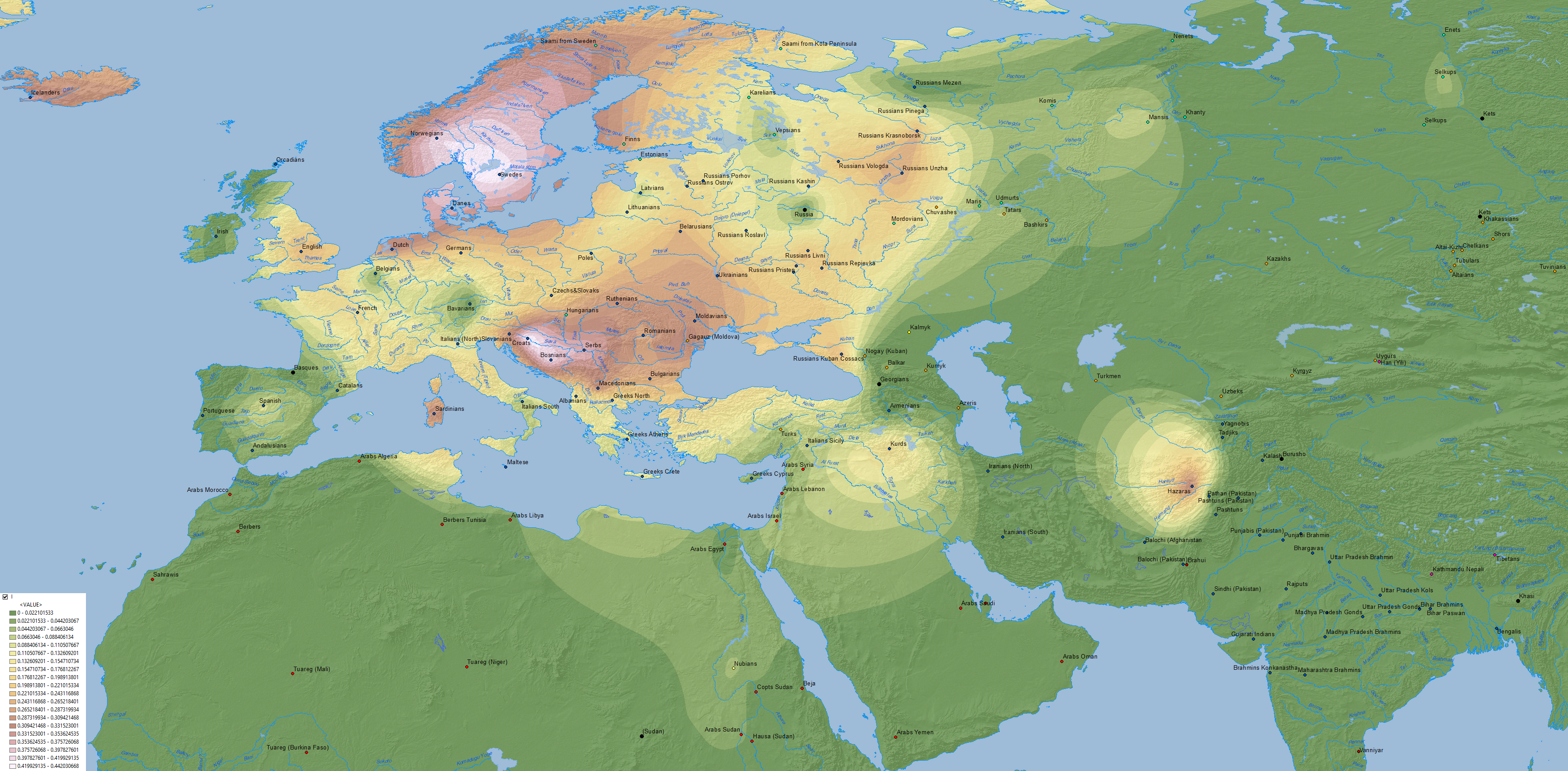
I actually don't think there is any phenotype difference across Estonia.

On this map you can see that Estonia has a fairly homogeneous admixture while Finland is divided.

So, you get Nordids, Baltids, Lapponoid-looking types and occasional Alpines all over the country.



I would try to suggest that it is haplogroup I that boosted West Estonian height.

[Russki]

Here's also a biplot of the populations, where each population is connected with a line to its two closest neighbors:



[/code]

Thank for your work.

Didn't the West Estonian type and the Curonian type come out too close on PCA for a rather huge hair color difference?

[Komintasavalta]

I actually don't think there is any phenotype difference across Estonia.

There is according to Juhan Aul's book "Антропология эстонцев": http://dspace.ut.ee/handle/10062/41630?show=full. And also according to Karin Mark's data, for example Southern Estonians have darker hair than Northern Estonians: https://www.etis.ee/Portal/Publicati...8-b9b3010eabad.

On this map you can see that Estonia has a fairly homogeneous admixture while Finland is divided.

I don't think Eupedia had Estonian regional averages for Dodecad K12b. I recently made Lithuanian regional averages for Eurogenes K13 though: https://www.theapricity.com/forum/sh...=1#post7331581.

Thank for your work.

Didn't the West Estonian type and the Curonian type come out too close on PCA for a rather huge hair color difference?

The colors don't have any particular significance, and I just assigned them randomly. The colored groups are based on cutting a hierarchical clustering tree at the height where it has 12 subtrees.

I wish I could post your table on the Finnish anthroforum, but I got banned from there... Finns have very little knowledge of the Soviet anthropological studies of Uralic peoples. But it's cool that on this forum there are users like you and travv and Lucasz, who keep bringing us gems from behind the Iron Curtain.

[sevruk]

The most big works on Russian anthropology are those of Deryabin (On Russian):
East Slavs
Дерябин славян&#10.zip
Caucasus and Western Asia
Kavkaz.zip