by Carl O. Nordling Finland is populated by three distinct ethnic groups which will be referred to as the (Finland-) Saamis, the Finns and the Finland-Swedes, respectively. The Finns speak a language closely related to Estonian, which is a reason for expecting a certain degree of genetic relationship as well. The Finland-Swedes speak the language of Sweden; this, too, constitutes a reason for looking for a genetic relationship. However, the solid blood group investigation of Nevanlinna (1973) made it dear that the Finns are genetically different from the Estonians, and that the Finland-Swedes differ from the Swedes in Sweden. Therefore, it is fairly obvious that both groups must be of mixed breeding.
In order to determine the proportions of genes from various sources in the current gene pool of a certain population, one or more mathematical methods are needed. The first method that presents itself for the purpose is the concept of the so-called genetic distance. This distance is measured as a kind of average of a number of gene-frequency differences between the two populations in question. (For simplicity's sake, I have used the square root of the mean of all the separate gene differences squared.) If a certain people, A, has genetic distances to two other peoples, B and C, which distances add up to the distance between B and C (or a little more), it would indicate the possibility of A being a mixed breed composed of genes from B and C. In the case of the Icelanders, for instance, their distances to the Norwegians and to the Irish add up to about twice the distance between the latter two. Consequently, the genetic distances do not mark the Icelanders as a mixed breed composed of Norwegians and Irishmen. Obviously, measuring genetic distances is not enough to solve the problem of determining the components of a mixed breed; but it may be a useful first step. At a stage when such components have been determined, distances may also be used to determine the proportions of the components. Nevanlinna (1973) has provided excellent statistics with frequency figures for 19 allele genes, distributed according to counties and language groups, covering all of Finland except the Saamis. Fortunately, comparable data are available for Estonia and for various parts of Sweden. One of my working hypotheses was that the counties that shared a common dialect would also share some genetic traits which would distinguish them from other dialect groups. It appeared that this
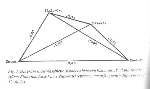
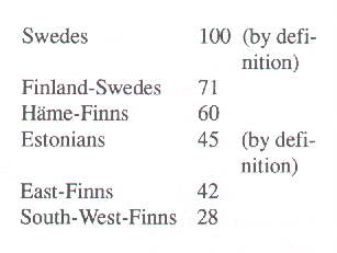
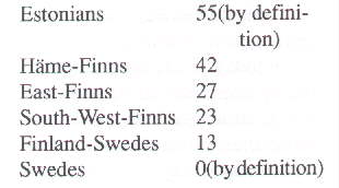
Figure 1 shows the genetic distances between four of the race groups concerned (Finland-Swedes, Häme-Finns, East-Finns and a sample group of Estonians) graphically. It appears that the Häme-Finns are not far from being a perfect match to a mixed breed between Finland-Swedes and East-Finns. However, there are reasons to suspect that the latter two groups are both of mixed breeding themselves; they may even have been compounded later than the Häme-Finns. Since the East-Finns obviously have less of the Swedish component than the Häme-Finns and the Finland-Swedes, one would expect them to be very close to their linguistic relatives, the Estonians. But astonishingly enough, the genetic distance between the Estonians and the East-Finns is the longest of all. Measuring genetic distances per se does not tell us how these race groups have been mixed together. That being the case, why not try the option introduced by Mark (1970), the "Europidity index "? According to the allele statistics of Ryman et al. (1981) the Swedes share with other Europeans a high frequency of - for instance - the allele genes N and P, which at the same time show lower frequencies among all the five groups under scrutiny here. If the frequency values of these two genes among the Swedes are given index values of 100 and the frequency values among the Estonians are given index values of, say, 45, we obtain the following provisory index values of "Europidity" for all our groups:
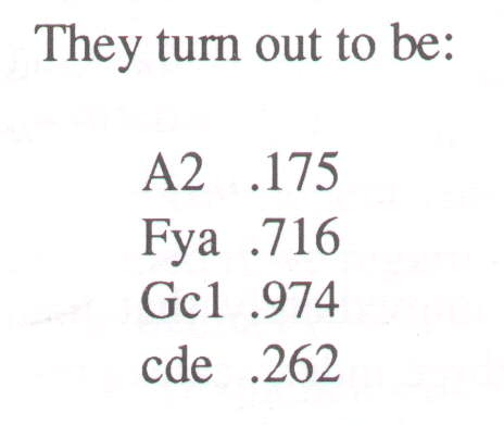
Since - to take one exampel - the East-Finns only rate 42 and 27 on the Europidity and Estonidity scales, respectively, there is reason to expect a third, unknown component in their gene pool. This unknown component must be characterized by rather extreme frequencies of certain alleles, especially A2, Fya, Gc1 and cde. The East-Finns rate higher than any other of the relevant groups in respect of the first three of these and rather low where cde is concerned.
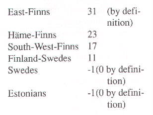
Clearly, than, "X " represents a Saami group - probably one found among the North-Eastern Saamis tat now populate parts of northern Finland and eastern Norway. Therefore, the natural next step would be to construct an "NE-Lappidity" index. We might let the frequency values of the alleles Fya, Gc1 and cde among the East-Finns have index values of 31 and the frequency values halfway between those of the Swedes and the Estonians have index values of zero, and all other values being assessed accordingly. This will produce the following provisory index values of "NE-Lappidity":
It must be noted immediately that the calibration of the three index scales presented above is not derived from any calculation. We have simply assumed that the Estonians rate 45 on Europidity and the East-Finns 31 on NE-Lappidity as a temporary device, If it can be proved that three genetic components will suffice to describe the composition of the gene pools of the groups under scrutiny, there still remains the problem of measuring the real proportions of these components. I have tried to solve the problem by means of constructing three hypothetical gene sets that may be blended together in various proportions to form acceptable copies of the gene sets of the East-Finns, the Häme-Finns, the South-West-Finns and the Finland-Swedes. At the same time, I have required that one of the hypothetical sets be typically Scandinavian, another typically NE-Lapponian and the third such that it will produce the established Estonian gene set when blended in the proportion 55 to 45 with the first set (the "Scandinavian" one). The attempt succeeded in part. Three hypothetical basic sets that meet the said requirements will indeed suffice to make good copies of the established gene sets of the East-Finns, the Häme-Finns and the Finland-Swedes. At the same time, though, it became quite clear that no mix of any three components fulfilling the requirements could possibly match the gene set of the South-West-Finns. The most likely explanation of this state of things is that the gene pool of the South-West-Finns contains not only the three components described above but also a fourth, unknown component. Identifying this component is of course a challenge. In order to make the three components appropriate for fonning the required gene sets of today, it was necessary to assume that the Scandinavian component should diverge rather markedly from the average frequencies among all groups of Swedes. (Certain subgroups usually do diverge |
|
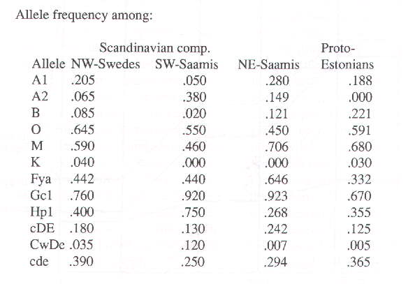
considerably from the average of the group as a whole.) By carefully studying the regional frequency tables of Beckman (1959), a possible explanation of this discrepancy was discovered; it turned out that the deviation from the frequencies among Swedes in general may be accounted for by means of assuming that the well-suited Scandinavian component is, in its turn, composed of one part genes from Swedish Saamis (SW-Saamis) and five parts genes from Swedes of the sub-group that now populates southern Norrland and northern Dalecarlia. In other words, the peculiarities of the Scandinavian component can be satisfactorily explained if we regard it as compounded in the manner described. The frequencies of 19 allele genes in all were used to test the hypothesis that the race groups in Finland are all composed of the same three components. Among these 19, there are 12 with frequencies that diverge enough for them to be crucial in the context. The further division of the Scandinavian component into two subcomponents has been tested with regard to the 12 crucial alleles. The calculated frequencies for these 12 genes in respect of each of the now four hypothetical primordial components are as follows: Allele frequency among:
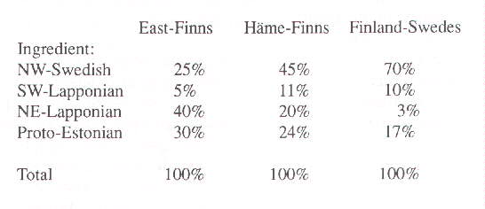
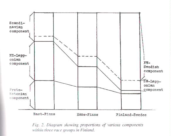
Given these four basic gene sets as ingredients at our disposal, we may now calculate the best recipe for blending proportions when it comes to making a copy of each of the gene sets of the East-Finns, the Häme-Finns and the Finland-Swedes. This calls for a procedure of successive trials and adjustments. So far, I have found the best recipes to be the following ones: See also Figure 2).
The numerical values should not be regarded as a true-to-life description of the genetic composition of the groups in question, because the proportions could easily be raised or lowered a little by slightly changing the frequency values of the components. The important thing is that no such tampenng would change the general pattern of genetic composition that has been deduced here. It is also important to point out that there exists no alternative theory that would describe the genetic composition of these race groups in some other way.
Beckman, L. 1959. A contribution to the physical anthropology and population genetics of Sweden. Variations of the ABO, Rh, MN and P blood groups. Hereditas 45. Mark, K. 1970. Zur Herkunft der Finnisch-ugrischen Völker vom Standpunkt der Anthropologie, Taflinn. Mourant, A.E., Kopec, A.C. & Domaniewska-Sobczak, K. 1976. The distribution of the human blood groups, London. Nevanlinna, H.R. 1973. Soumen väestörakenne. Kansaneläkelaitoksen julk. A. 9. Helsinki. Ryman, N. et al. 1981. Probability of paternity exclusion in different mother-child genotype combinations. Hereditas 94. |